I’ve lately written about Impermanent Loss (“IL”) and how it’s primarily the identical factor as Loss Versus Rebalancing (“LVR”) and in the middle of discussing it (thanks Alex) I spotted that we outlined IL badly. I’ll right here redraw the arguments made on this submit in a extra thorough method, and supply an improved definition of IL, or moderately DL (for Divergence Loss), as a result of underneath the brand new definition there’s nothing impermanent with this loss. For extra in-depth rationalization of a number of the methods employed right here — notably on the linkage between AMMs and choice pricing — I like to recommend to learn my paper on theammbook.org first, particularly chapter 4.
The IL is at the moment outlined because the alternative loss towards HODL, ie the distinction of the 50/50 preliminary place merely held, and the worth of the AMM place. If the outline xi because the ratio between the worth now and the worth when the place was entered into, then IL is

If costs return to the unique level then xi=1 and subsequently the loss turns into zero — therefore the moniker “Impermanent”. Individuals have identified that there’s nothing impermanent about this loss if costs don’t return to their preliminary worth— as one hopes on a pool like WBTC/USDC the place one expects for WBTC to moon — and subsequently the time period “Divergence Loss” or “DL” was coined. We are going to see under that correctly outlined “IL” is non-zero even when xi returns to be unity, subsequently we are going to drop the IL moniker from this level onwards and refer completely to DL.
To grasp the difficulty with the present definition of DL, I first need to return to the fundamentals and take into account a set revenue funding — say $100 when charges are at 5%. If I give these $100 away and I get $100 again in a yr threat free (no upside, no draw back), then I emphatically didn’t break even: at 5% curiosity I ought to have gotten again $105, so if I made a lack of $5. I’ll now present that the identical factor applies for an CFMM liquidity place: it ought to make develop over time, and after a yr if xi returns to 1 I ought to get again 1+r instances my preliminary funding with the speed r>0 to be decided under. If I solely get again my funding, my loss ratio is r.
So how a lot ought to an funding into an AMM liquidity place earn? The tactic I exploit may be utilized universally, however for simplicity I’ll limit myself to a CFMM, ie ok=x*y, and I’ll assume that the pool is ETH/USDC for ease of language. On this case it’s well-known that (assuming environment friendly markets all through this paper)
- at any level of time, the worth of the ETH place is precisely the identical as that of the USDC place; this holds for each numeraire, however for simplicity I assume “greenback worth”
- if the place was contributed at a normalized worth ratio of xi=1, then at any time limit sooner or later, the worth of the whole place is proportional to sqrt(xi)
One of the best framework for analyzing AMMs is that of a self-financing buying and selling technique. The latter is outlined as a time various multi-asset place (presumably lengthy and quick), the place the worth of the place solely adjustments due to market strikes. Importantly, no property are to be added or eliminated, they’ll solely be traded. On this case, buying and selling should occur at precisely the present market worth, subsequently buying and selling doesn’t impression the worth of the portfolio. Due to level (1) above, it’s clear that an AMM LP place may be thought-about a repeatedly rebalanced technique that ensures that at any level of time 50% of the portfolio worth is in ETH and 50% in USDC.
To point out that this means (2), it’s simpler to go backwards: we assume that we’ve got a method whose worth at any time is ok(t) sqrt(S) the place S is the spot change fee (and, for reference, xi=S(t)/S(0)). If we delta hedge this profile then the Money Delta (see right here, part 4) is CashDelta = S d/dS sqrt(S) and it’s simple to see that additionally CashDelta = 0.5 sqrt(S). In different phrases: when delta hedging the sq. root profile, at any time limit 50% of the money is invested within the threat asset, and subsequently the opposite 50% within the numeraire. Subsequently the 50/50 technique is the replicating technique for the sq. root profile. /QED
I’ve proven right here (part 4.3) that the Black Scholes constituent operators are diagonal on energy regulation capabilities, ie if we’ve got

then the constituent differential operators of the Black Scholes PDE turns into diagonal

and subsequently the Black Scholes PDE simplifies on this eigen foundation to the next abnormal differential equation (ODE)

Notice that the time period in parentheses is only a fixed, so this ODE is of the well-known type f’ = kf, and we all know that the answer to this ODE is solely f(t)=f(0) exp(kt).
The sq. root profile is the facility regulation perform at alpha=0.5, so we will plug in 0.5 into the above equation to get the issue ok which turns into
ok = sigma²/8 + 0.5(r-d)+r
Assuming zero charges, and shifting to the decay time scale tau = 1/ok we discover

and

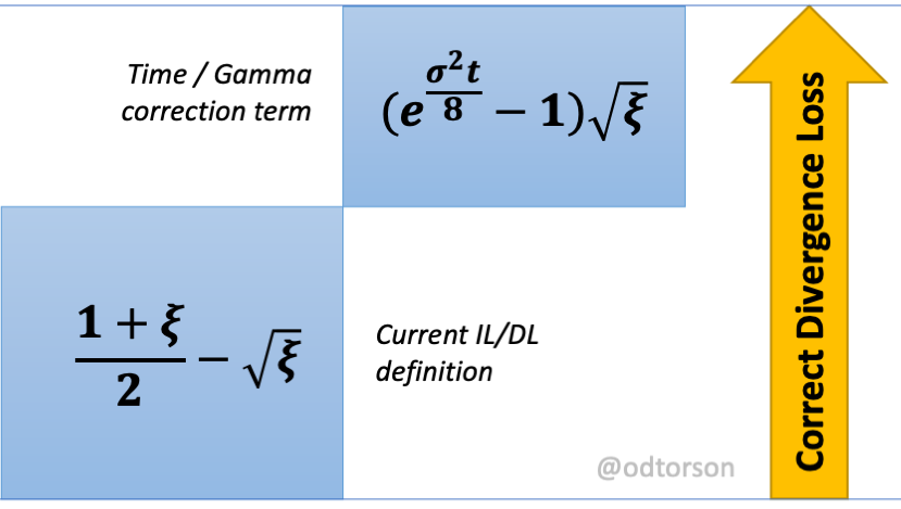
Now we’ve got all we have to outline Divergence Loss correctly. The important thing perception right here is that an CFMM funding technique — 50/50 in every asset — ought to yield a return of exp(t/tau) sqrt(xi). As an alternative it yields sqrt(xi). That is an outright loss, akin to the “getting again $100 after a yr at 5% charges” state of affairs mentioned above. Subsequently the DL has two elements
- the distinction between HODL and the CFMM worth, and
- the distinction between the CFMM worth and the honest worth of the 50/50 self financing funding technique

In abstract, the Gamma / time correction time period — equivalent to the Gamma revenue a 50/50 technique ought to make — is an integral a part of the calculation of the Divergence Loss. Together with this time period makes Divergence Loss strictly better than zero for t>0, subsequently the moniker Impermanent Loss is not enough. When calculating DL on this approach it’s equal to the LVR measure, with the DL being the macroscopic measure, and the LVR being the equal infinitesimal measure.